
Control Strategies Used in Smart Buildings
28 October 2020 by Sergio Durán
Buildings are where daily life happens — homes, offices, hospitals, leisure centers, and more. Keeping these facilities comfortable, functional, and continuously operational comes at a significant energy cost.
The International Energy Agency (IEA) reports that buildings and the construction sector account for one-third of global energy consumption and roughly 40% of worldwide CO₂ emissions — and demand continues to grow [1].
Over the past several years, a new generation of buildings has emerged: ones with integrated automation systems for HVAC, lighting, security, multimedia, and telecommunications, all managed remotely with the goal of improving energy efficiency and usability. These are smart buildings.
Achieving the right level of automation requires selecting and tuning the correct control strategy for each system. Below are the most common strategies used in smart building applications.
ON/OFF Control
ON/OFF control is exactly what it sounds like: the controller switches between two states, on and off. It is the simplest and least precise control strategy. Its operating principle relies on a reference setpoint and feedback from the plant (the process being controlled).
When the feedback variable falls below the setpoint, the controller turns the plant on; when it rises above it, the controller turns the plant off. This switching behavior causes the system output to oscillate continuously. Despite its limitations, ON/OFF control is the most cost-effective option and is widely used in temperature control systems.
A practical refinement is to treat the setpoint as a reference band rather than a single value, which reduces high-frequency oscillation and prevents equipment wear. It is also worth accounting for hysteresis in mechanical sensors, which affects the amplitude and frequency of that oscillation.
Hysteresis is the tendency of some materials to "remember" a previous state. In this context, it creates an asymmetry between the time the process stays on versus off, effectively lengthening the oscillation period. If a constant output is required, a more precise strategy is a better fit.
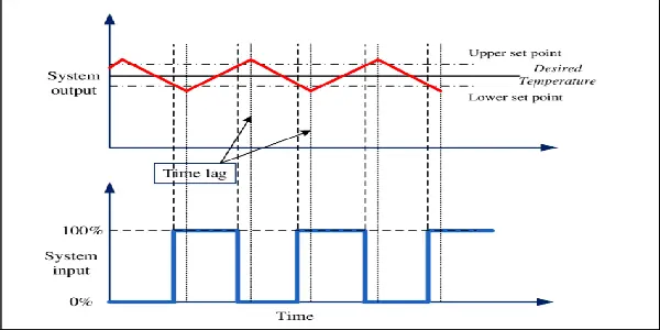 Typical oscillatory behavior of an ON/OFF control system.
Proportional Control
Proportional control is another widely applied technique. Like ON/OFF, it operates with feedback — but instead of switching between two states, it amplifies the error signal by a variable gain to regulate the plant toward a defined setpoint.
In a smart building, proportional control is typically applied to systems such as water tank fill/drain management and temperature regulation. Its mathematical expression is:
Y(t) = Kp * e(t)
PID Control
The PID controller — proportional, integral, and derivative — is an optimized extension of proportional control. It is a closed-loop strategy that regulates the output variable with considerably higher precision, and it is the most widely used control strategy across industry.
In building automation, its main applications include dynamic artificial lighting control (balanced against available daylight), temperature regulation, airflow speed control in HVAC systems, pump control, and water heating system temperature management.
The controller works by calculating the difference between the setpoint and the feedback signal, then producing a corrective output to keep the plant at a steady value. Its governing equation is:
Y(t) = Kp*e(t) + Ki * ∫e(t)dt + Kd * de(t)/dt
Proportional Term
The proportional term represents the instantaneous difference between the actual and desired values — it drives the system toward the setpoint by minimizing the error. This behavior is tuned by adjusting the constant Kp.
Increasing Kp raises the system's response speed and reduces steady-state error, but also increases instability. Because the proportional term ignores time-based variations, instability is best corrected by adjusting the integral and derivative terms rather than Kp alone.
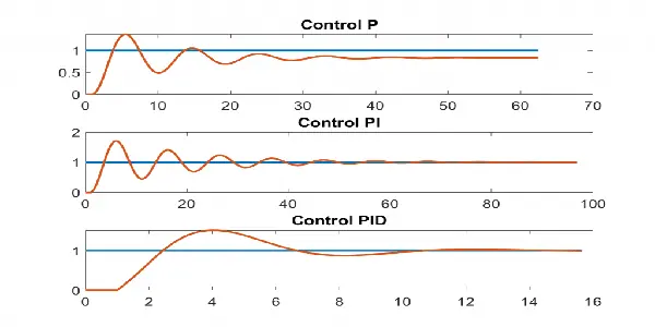 Typical PID controller response with all three terms active.
Integral Term
The integral term tracks the cumulative error over time, building up the corrective action needed to eliminate persistent steady-state error. Its tuning constant is Ki.
Increasing Ki reduces steady-state error and modestly increases system speed, but at the cost of reduced stability. Careful tuning is required to balance these trade-offs.
Derivative Term
The derivative term predicts how quickly the error is changing and applies a corrective action ahead of time. Without it, proportional and proportional-integral controllers tend to overshoot the setpoint and oscillate before settling.
The derivative term essentially senses how fast the actual value is approaching the setpoint and begins to ease off before it gets there, reducing overshoot. Increasing Kd improves system stability and has no effect on steady-state error, though it slightly reduces response speed.
Real-World Constraints
Physical systems always impose limits on how aggressively a controller can be tuned. Consider a building's water heating system: if the heating element has a maximum capacity of 1,500 W, progressively increasing Kp to speed up the response will eventually saturate the controller — the heater simply cannot exceed its power limit.
This is why understanding the real operating constraints of the system is a prerequisite for designing any PID controller, not an afterthought.
Sergio Durán Development Engineer sduran@innotica.net · LinkedIn